Timeseries

---

Introduction of time series

What makes timeseries special is that the data is not necessarily independent and not necessarily identically distributed compare to the standard linear regression.

Also the time series has the time index or we can say the list of observations where ordering maters. Ordering is important here, since it affect the meaning of the data.

Autocorrelation Function

The autocorrelation function (ACF) for a series is to find the correlations between series $x_t$ and lagged values of the series such like $x_{t-1}, x_{t-2},...$.

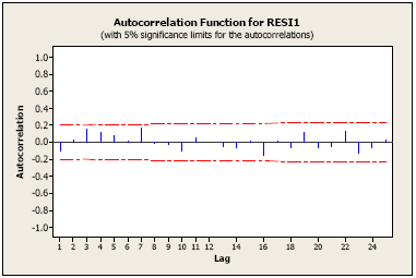
The ACF can be used to identify the structure of our time series data. In addition, the ACF of the residuals in a model is also useful. The idea is that we do not want to see any siginificant correlation for any lag in the ACF of the residual.

The figure above is the ACF for a AR(1) residual, the blue vertical lien is the autocorrelation at each lag. The red horizontal line is the statistic significant bounds. In this figure, nothing is significant which is good.

Stationary Series

To make our ACF meaningful, we need have a weakly stationary series .This means the autocorrelation is same for any lag regardless of the time.

(weakly) Stationary Series satisfies the following properties:

• The mean $E(x_t)$is the same for all time $t$
• The variance of $x_t$ is hte same for all $t$
• The covariance and correlation between $x_t$ and $x_{t-1}$ is the same for all $t$

For a ACF between $x_t$ and $x_{t-h}$:

$\frac{Cov(x_t, x_{t-h})}{sd(x_t)sd(x_{t-h})} = \frac{Cov(x_t, x_{t-h})}{sd(x_t)}$

The reason that we can write the denominator in the right hand side in the above formula is we have wwakly stationary series.

In the real world data, most of them are not stationary. Especially, the trend in our data against the property that have same mean for all $t$. Also the distinct seasonal pattern also against the requirement.

Autoregression Model

Also called AR§ model. When $p=1$ as the 1st order autoregressive model is denoted as AR(1):

$x_t = \delta + \phi_1 x_{t-1} + \omega_t$

• Where $\omega+y \sim N(0, \sigma^2_\omega)$ means the error is iid and has mean 0 and constant variance.
• properties of errors $\omega_t$ are independent of $x_t$
• $x_1, .., x_t$ is weakly stationary.

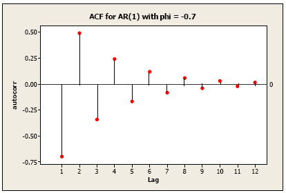
These two type of ACF plot, the first plot indicated we have a positive value of $\phi_1$ since the acf is exponentially decrease to 0 as lag h increase. The second plot with alternate sign indicate we have a negative $\phi$

Moving Average

Let the $w_t \sim N(0, \sigma^2_w)$,

The 1st order moving average model is MA(1):

$x_t = \mu +w_t +\theta_1w_{t-1}$

MA(2):

$x_t = \mu +w_t + \theta_1w_{t-1} +\theta_2w_{t-2}$

ARIMA-autoregreesive integrated moving average

Before we select the model, we need to test the stationarity of the data. A time series is stationary if it has constant mean and variance, and covariance is independent of time. The test I used is Dickey-Fuller test, the null hypothesis is that a unit root exists. If there is a unit root exists, then $p > \alpha$, we say the process is not stationary at $\alpha$ significant level.

In the common time series model, we have autoregressive (AR) model–AR§, moving average (MA) model–MA(q), autoregressive–moving-average (ARMA)–ARMA(p,q) and Autoregressive integrated moving average (ARIMA)–ARIMA(p,d,q) where p,d,q stands for seasonality, trend, and noise in data.

• AR: Auto-Regressive §: AR terms are just lags of dependent variable. For example lets say p is 3, we will use x(t-1), x(t-2) and x(t-3) to predict x(t)
• I: Integrated (d): These are the number of non-seasonal differences. For example, in our case we take the first order difference. So we pass that variable and put d=1
• MA: Moving Averages (q): MA terms are lagged forecast errors in prediction equation.

The way I use find the suitable model is to try to look at autocorrelation and partial-autocorrelation which will give us a first idea to select the range of parameters. Then based on the AIC(Akaike information criterion) which can define the goodness of a model, to test the parameter.

In the test, we found that the original time series is not stationary. Then we can try the first order difference and try to look at weekly data to get more smooth trend.

To find the better parameter, we can use AIC or BIC. But note that, when models are compared using these values, it is important that all models have the same orders of differencing. If a model has a order of differencing (d) of a model, then the data is changed on which the likelihood is computed, making the AIC values between models with different orders of differencing not comparable.

Seasonal autoregressive integrated moving average model(SARIMA)

SARIMA (p,d,q) * (P,D,Q,S) where (p,d,q) is same as ARIMA (These three parameters account for seasonality, trend, and noise in data), and P is the seasonal autoregressive component, D is the seasonal difference, Q is the seasonal moving average component, S is the length of the season.

The general formula for SARIMA with seasonal period as 12(months per year) is:

where

Since we already find there is a seasonal part in our data, then seasonal differencing will be used. The data we used later is the linear combination of the few Keywords and Heat Index between 2017/01/01 to 2019/07/13.

To compare each model with different parameter, I used log-likelihood to find out the better parameter in ARIMA. Smaller log-likelihood, AIC or BIC means this model is better.

Some comparison:

ARIMA model	mean square error
ARIMA(3,0,1)(2,1,2,12)	275
ARIMA(3,1,2)(2,1,2,12)	279
ARIMA(3,0,2)(0,1,2,12)	260
ARIMA(3,0,2)(1,1,2,12)	266
ARIMA(3,0,1)(1,1,2,12)	276
ARIMA(2,0,1)(0,1,2,12)	268
ARIMA(2,1,1)(0,1,2,12)	271
ARIMA(2,1,1)(0,1,2,12)	271
ARIMA(3,1,1)(0,1,2,12)	270

…

Then ARIMA(3,0,2)(0,1,2,12) may be better here.