Classification

Logistic Regression

Note that Logistice regression is not a regression problem but a classification problem. The most simple one is binary classification. One method is to use linear regression to map all predictors bigger than 0.5 as 1 and less than 0.5 as 0. But this can not work very well since it is not a linear function.

Hence we used Sigmoid Function: $0\leq h_\theta(x) \leq1$

$\begin{aligned} h_\theta(x) &= g(\theta^Tx) \\ z &= \theta^T x \\ g(z) &= \frac{1}{1+e^{-z}} \end{aligned}$

The figure above is g(z)

Note that:

• There should be no outliers in the data, which can be assessed by converting the continuous predictors to standardized scores, and removing values below -3.29 or greater than 3.29. (z-score)
• There should be no high correlations (multicollinearity) among the predictors. This can be assessed by a correlation matrix among the predictors.

$logit(p) = log(\frac{p}{1-p})$

Overfitting

When selecting the model for the logistic regression analysis, another important consideration is the model fit. Adding independent variables to a logistic regression model will always increase the amount of variance explained in the log odds (typically expressed as R²). However, adding more and more variables to the model can result in overfitting, which reduces the generalizability of the model beyond the data on which the model is fit.

K-NN (K-nerest neighbor)

It is supervised learning method. When we have a training set, after we got a new data we try to find the most nearest k data. In this k data, we find the highest frequency class to be the class of this new data. The distance between each point can be visit in “Distance or Similarity”.

Naive Bayesian Classifier

Bayesian rule:

$p(A|B)=\frac{p(B|A)p(A)}{p(B)}$

And it assumes that all features are independent which is a strong assumption.

Advantage:

• When it has small amount of training data, it has good predict power
• Training is fast, since calculate prior and likelihood is quick. Especially, if our assumption is hold.
• Highly scalable. It scales linearly with the number of features and data points and can be easily updated with new data

Disadvantage:

• Cannot incorporate feature interactions
• It is not good for continues data, since it can not calculate the accurate likelihoods
• It is very sensitive to the training data. For example, if the training data can not represent the distribution of the whole data, the priors will be incorrect

SVM

Support Vector Machine

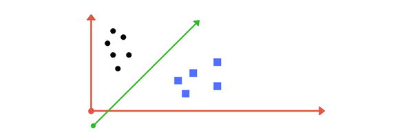
Support Vector is the line between two closest points where this line can separate these 2 points very well(vertical to the line connect these 2 points).

Also we have some restriction:

• number of features should less than the number of data. Treat this SVM problem as several function ($f(x)>0$ or $f(x)<0$) that we need to calculate whether a point is big or less than 0. The number of functions should large than the number of variables which equal to the restriction above.

• It is used for linear separable data problem. For nonliner problem, we can use kernel function to map the non-liner data into a linear separable problem